Stage-Two Filamentary Coil Optimization
This notebook will show how to use DESC to perform stage two coil optimization with filamentary coils of differing parameterizations, such as Fourier in terms of arbitrary angle (as pioneered by FOCUS) or planar coils described in terms of the coil center, normal to the plane, and a Fourier series describing the radius of the coil in that plane. We will first find a coilset for the precise QA (Landreman & Paul 2022) vacuum equilibrium, starting from an initial coilset composed of circular planar coils, with only coils parameterized by a Fourier series in an arbitrary curve parameter. A second coil optimization will be performed for a W7-X-like finite beta equilibrium using a coilset composed of various coil parameterizations. Once optimized, the normal field error will be assessed, and for the vacuum equilibrium, field line tracing will be performed to compare the Poincare trace to the equilibrium flux surfaces.
[3]:
import sys
import os
sys.path.insert(0, os.path.abspath("."))
sys.path.append(os.path.abspath("../../../"))
[ ]:
# from desc import set_device
# set_device("gpu")
As mentioned in DESC Documentation on performance tips, one can use compilation cache directory to reduce the compilation overhead time. Uncomment the next code block to take advantage of the cache.
Note: One needs to create jax-caches folder manually.
[5]:
# import jax
# jax.config.update("jax_compilation_cache_dir", "../jax-caches")
# jax.config.update("jax_persistent_cache_min_entry_size_bytes", -1)
# jax.config.update("jax_persistent_cache_min_compile_time_secs", 0)
[6]:
import numpy as np
from desc.backend import print_backend_info
from desc.coils import (
CoilSet,
FourierPlanarCoil,
MixedCoilSet,
initialize_modular_coils,
initialize_saddle_coils,
)
import desc.examples
from desc.equilibrium import Equilibrium
from desc.plotting import plot_2d, plot_3d, plot_coils, plot_comparison
from desc.grid import LinearGrid
from desc.objectives import (
ObjectiveFunction,
CoilCurvature,
CoilLength,
CoilCurrentLength,
CoilTorsion,
CoilSetLinkingNumber,
CoilSetMinDistance,
LinkingCurrentConsistency,
PlasmaCoilSetMinDistance,
QuadraticFlux,
ToroidalFlux,
FixCoilCurrent,
FixParameters,
)
from desc.optimize import Optimizer
from desc.integrals import compute_B_plasma
import time
import plotly.express as px
import plotly.io as pio
# This ensures Plotly output works in multiple places:
# plotly_mimetype: VS Code notebook UI
# notebook: "Jupyter: Export to HTML" command in VS Code
# See https://plotly.com/python/renderers/#multiple-renderers
pio.renderers.default = "plotly_mimetype+notebook"
print_backend_info()
DESC version=0.16.0+72.g14d4554c4.dirty.
Using JAX backend: jax version=0.6.2, jaxlib version=0.6.2, dtype=float64.
Using device: NVIDIA GeForce RTX 4080 Laptop GPU (id=0), with 11.60 GB available memory.
Coil Optimization Metrics
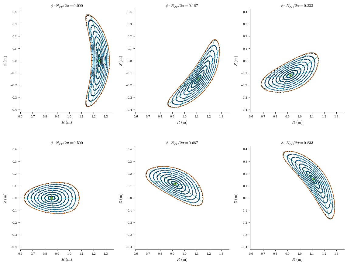
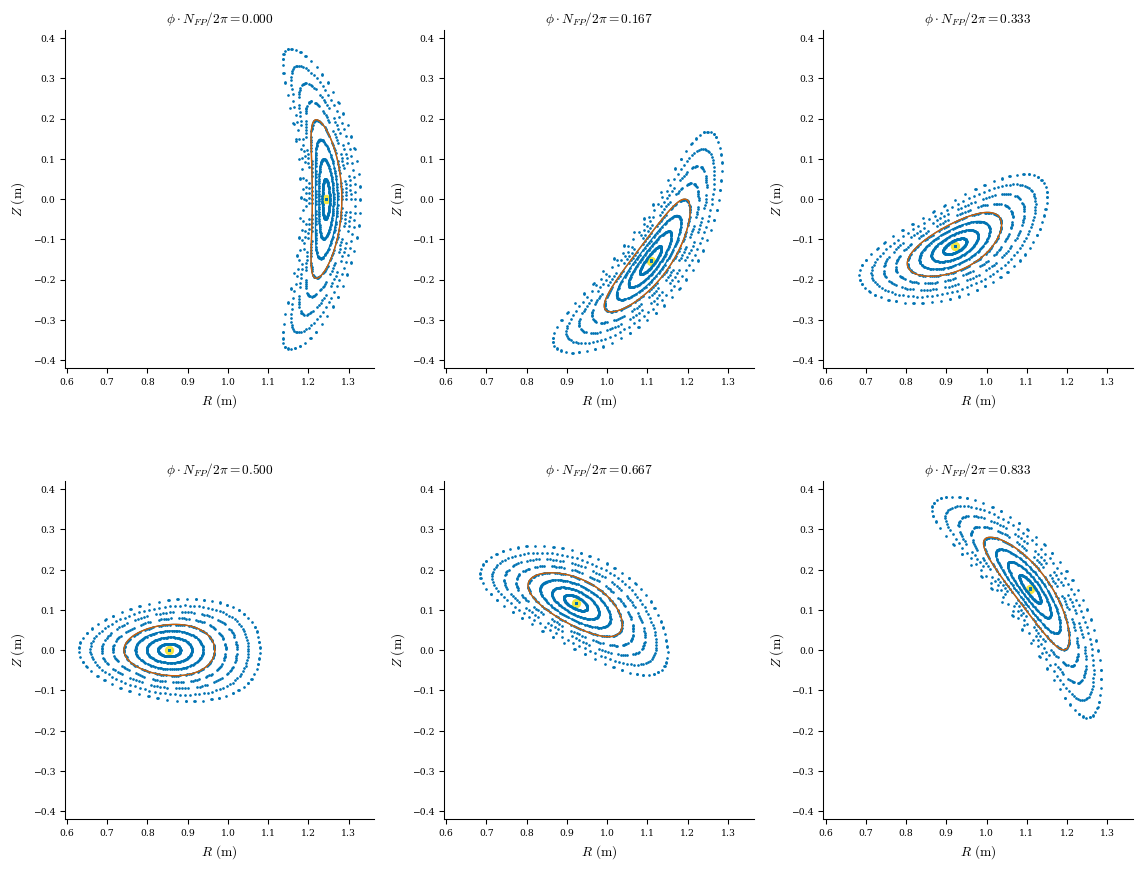
Two main figures of merit regarding the quality of the coil optimization in recreating the equilibrium are the average normalized magnetic field and Poincare plot from the coils. The average normalized magnetic field is a measure of how well the coils’ field (plus the plasma field if it is finite beta) recreates last closed flux surface of the target equilibrium and is given as
where \(\mathbf{\hat{n}}\) is the normal vector to the equilibrium’s last closed flux surface and \(\mathbf{B}_{\text{total}} = \mathbf{B}_{\text{coils}} + \mathbf{B}_{\text{plasma currents}}\). Field traces are also significant for vacuum equilibria because they visually show the quality of the coil field in recreating the equilibrium vacuum flux surfaces.
These two metrics are calculated in functions below.
[7]:
def compute_average_normalized_field(
field, eq, vacuum=False, chunk_size=None, B_plasma_chunk_size=None
):
if B_plasma_chunk_size is None:
B_plasma_chunk_size = chunk_size
grid = LinearGrid(M=80, N=80, NFP=eq.NFP)
if vacuum:
# we can avoid the expensive plasma contribution calculation if we
# just pass in the surface instead of the Equilibrium!
Bn, surf_coords = field.compute_Bnormal(
eq.surface,
eval_grid=grid,
chunk_size=chunk_size,
B_plasma_chunk_size=B_plasma_chunk_size,
)
else:
Bn, surf_coords = field.compute_Bnormal(
eq,
eval_grid=grid,
chunk_size=chunk_size,
B_plasma_chunk_size=B_plasma_chunk_size,
)
normalizing_field_vec = field.compute_magnetic_field(surf_coords)
if not vacuum:
# add plasma field to the normalizing field
normalizing_field_vec += compute_B_plasma(
eq, eval_grid=grid, chunk_size=B_plasma_chunk_size
)
normalizing_field = np.mean(np.linalg.norm(normalizing_field_vec, axis=1))
return np.mean(np.abs(Bn)) / normalizing_field
def plot_field_lines(field, eq):
# for starting locations we'll pick positions on flux surfaces on the outboard midplane
grid_trace = LinearGrid(rho=np.linspace(0, 1, 9))
r0 = eq.compute("R", grid=grid_trace)["R"]
z0 = eq.compute("Z", grid=grid_trace)["Z"]
fig, ax = desc.plotting.plot_surfaces(eq)
fig, ax, data = desc.plotting.poincare_plot(
field, r0, z0, NFP=eq.NFP, ax=ax, color="k", size=1, return_data=True
)
return fig, ax, data
Vacuum
We will be focusing on optimizing coils with the vacuum precise QA as the target equilibrium.
[8]:
eq = desc.examples.get("precise_QA")
Make initial coilset
We start by creating planar coils centered and aligned with the magnetic axis, equally spaced in the toroidal angle phi. Note that the coil positions are chosen to avoid the symmetry planes. We then convert the planar coils to the FourierXYZ parameterization. There are only 3 “unique” coils, and the full CoilSet accounts for the other “virtual” coils from field period and stellarator symmetry.
[9]:
coilset = initialize_modular_coils(eq, num_coils=3, r_over_a=3.0).to_FourierXYZ()
# visualize the initial coilset
# we use a smaller than usual plot grid to reduce memory of the notebook file
plot_grid = LinearGrid(M=20, N=40, NFP=1, endpoint=True)
fig = plot_3d(eq, "|B|", grid=plot_grid)
fig = plot_coils(coilset, fig=fig)
fig.show()
/CODES/DESC/desc/utils.py:572: UserWarning:
Unequal number of field periods for grid 1 and basis 2.
/CODES/DESC/desc/utils.py:572: UserWarning:
Unequal number of field periods for grid 1 and basis 2.
Optimizing a FourierXYZCoil coil set
[10]:
# number of points used to discretize coils. This could be different for each objective
# (eg if you want higher resolution for some calculations), but we'll use the same for all of them
coil_grid = LinearGrid(N=50)
# similarly define a grid on the plasma surface where B*n errors will be evaluated
plasma_grid = LinearGrid(M=25, N=25, NFP=eq.NFP, sym=eq.sym)
# define our objective function (we will use a helper function here to make it easier to change weights later)
weights = {
"quadratic flux": 200,
"coil-coil min dist": 100,
"plasma-coil min dist": 10,
"coil curvature": 750,
"coil length": 20,
}
def make_vac_coil_obj(eq, coilset, weights_dict):
obj = ObjectiveFunction(
(
QuadraticFlux(
eq,
field=coilset,
# grid of points on plasma surface to evaluate normal field error
eval_grid=plasma_grid,
field_grid=coil_grid,
vacuum=True, # vacuum=True means we won't calculate the plasma contribution to B as it is zero
weight=weights_dict["quadratic flux"],
bs_chunk_size=10,
),
CoilSetMinDistance(
coilset,
# in normalized units, want coil-coil distance to be at least 10% of minor radius
bounds=(0.1, np.inf),
normalize_target=False, # we're giving bounds in normalized units
grid=coil_grid,
weight=weights_dict["coil-coil min dist"],
dist_chunk_size=2, # this helps to reduce peak memory usage, needed to run on github CI
),
PlasmaCoilSetMinDistance(
eq,
coilset,
# in normalized units, want plasma-coil distance to be at least 25% of minor radius
bounds=(0.25, np.inf),
normalize_target=False, # we're giving bounds in normalized units
plasma_grid=plasma_grid,
coil_grid=coil_grid,
eq_fixed=True, # Fix the equilibrium. For single stage optimization, this would be False
weight=weights_dict["plasma-coil min dist"],
dist_chunk_size=2, # this helps to reduce peak memory usage, needed to run on github CI
),
CoilCurvature(
coilset,
# this uses signed curvature, depending on whether it curves towards
# or away from the centroid of the curve, with a circle having positive curvature.
# We give the bounds normalized units, curvature of approx 1 means circular,
# so we allow them to be a bit more strongly shaped
bounds=(-1, 2),
normalize_target=False, # we're giving bounds in normalized units
grid=coil_grid,
weight=weights_dict["coil curvature"],
),
CoilLength(
coilset,
bounds=(0, 2 * np.pi * (coilset[0].compute("length")["length"])),
normalize_target=True, # target length is in meters, not normalized
grid=coil_grid,
weight=weights_dict["coil length"],
),
)
)
return obj
obj = make_vac_coil_obj(eq, coilset, weights)
## define our constraints
# we will constrain the current of one coil to avoid the trivial quadratic flux minimizing solution
# of zero coil current
coil_indices_to_fix_current = [False for c in coilset]
coil_indices_to_fix_current[0] = True
constraints = (FixCoilCurrent(coilset, indices=coil_indices_to_fix_current),)
# Alternatively, we could have used
# constraints = (ToroidalFlux(eq, coilset, eq_fixed=True),)
# to target the actual toroidal flux from the equilibrium, or
# constraints = (FixSumCoilCurrent(coilset),)
# to fix the sum of all the coil currents but as this is a vacuum calculation
# the specific value of the flux doesn't matter, we can always rescale the coil currents later.
# Pick an optimizer. For this problem with only linear constraints we can use a regular least squares method.
# if we used the ToroidalFlux constraint we would need to use a constrained optimization method
optimizer = Optimizer("lsq-exact")
(optimized_coilset,), _ = optimizer.optimize(
coilset,
objective=obj,
constraints=constraints,
maxiter=100,
verbose=3,
ftol=1e-4,
copy=True,
)
Building objective: Quadratic flux
Precomputing transforms
Timer: Precomputing transforms = 1.69 sec
Building objective: coil-coil minimum distance
Building objective: plasma-coil minimum distance
Building objective: coil curvature
Precomputing transforms
Timer: Precomputing transforms = 142 ms
Building objective: coil length
Precomputing transforms
Timer: Precomputing transforms = 4.04 ms
Timer: Objective build = 3.22 sec
Building objective: fixed coil current
Building objective: fixed shift
Building objective: fixed rotation
Timer: Objective build = 281 ms
Timer: LinearConstraintProjection build = 2.23 sec
Number of parameters: 191
Number of objectives: 1656
Timer: Initializing the optimization = 5.80 sec
Starting optimization
Using method: lsq-exact
Solver options:
------------------------------------------------------------
Maximum Function Evaluations : 501
Maximum Allowed Total Δx Norm : inf
Scaled Termination : True
Trust Region Method : qr
Initial Trust Radius : 1.499e+03
Maximum Trust Radius : inf
Minimum Trust Radius : 2.220e-16
Trust Radius Increase Ratio : 2.000e+00
Trust Radius Decrease Ratio : 2.500e-01
Trust Radius Increase Threshold : 7.500e-01
Trust Radius Decrease Threshold : 2.500e-01
------------------------------------------------------------
Iteration Total nfev Cost Cost reduction Step norm Optimality
0 1 4.516e+06 1.615e+03
1 7 4.504e+06 1.175e+04 5.310e-03 1.607e+03
2 8 4.479e+06 2.520e+04 6.741e-03 1.590e+03
3 9 4.435e+06 4.409e+04 6.494e-03 1.530e+03
4 10 4.355e+06 7.997e+04 4.127e-03 1.504e+03
5 11 4.200e+06 1.548e+05 8.231e-03 1.453e+03
6 12 3.926e+06 2.736e+05 1.375e-02 1.380e+03
7 13 3.425e+06 5.011e+05 2.741e-02 1.274e+03
8 14 2.578e+06 8.472e+05 5.426e-02 1.087e+03
9 15 1.364e+06 1.215e+06 1.048e-01 7.675e+02
10 16 2.933e+05 1.070e+06 1.943e-01 2.298e+02
11 17 2.382e+05 5.506e+04 2.969e-01 4.891e+02
12 18 3.409e+04 2.041e+05 5.565e-02 8.285e+01
13 19 1.077e+04 2.332e+04 1.215e-01 4.716e+01
14 20 8.098e+03 2.673e+03 2.462e-01 5.542e+01
15 22 1.234e+03 6.864e+03 5.484e-02 2.417e+01
16 23 6.630e+02 5.711e+02 1.247e-01 1.907e+01
17 25 3.501e+02 3.129e+02 2.962e-02 4.980e+00
18 26 2.015e+02 1.486e+02 3.069e-02 3.997e+00
19 28 1.436e+02 5.789e+01 7.511e-03 7.263e-01
20 29 1.265e+02 1.712e+01 1.584e-02 4.958e-01
21 30 9.738e+01 2.909e+01 3.217e-02 4.274e-01
22 32 8.725e+01 1.013e+01 1.599e-02 3.386e-01
23 34 8.034e+01 6.910e+00 7.940e-03 7.085e-02
24 36 7.794e+01 2.393e+00 3.986e-03 8.089e-02
25 37 7.333e+01 4.612e+00 7.983e-03 3.494e-02
26 40 7.278e+01 5.526e-01 9.963e-04 3.688e-02
27 41 7.169e+01 1.092e+00 1.990e-03 3.626e-02
28 44 7.155e+01 1.350e-01 2.487e-04 3.621e-02
29 47 7.153e+01 1.686e-02 3.109e-05 3.620e-02
30 48 7.150e+01 3.370e-02 6.217e-05 3.618e-02
31 51 7.150e+01 4.211e-03 7.772e-06 3.618e-02
Optimization terminated successfully.
`ftol` condition satisfied. (ftol=1.00e-04)
Current function value: 7.150e+01
Total delta_x: 1.177e+00
Iterations: 31
Function evaluations: 51
Jacobian evaluations: 32
Timer: Solution time = 26.2 sec
Timer: Avg time per step = 821 ms
==============================================================================================================
Start --> End
Total (sum of squares): 4.516e+06 --> 7.150e+01,
Maximum absolute Boundary normal field error: 1.656e-01 --> 9.435e-04 (T m^2)
Minimum absolute Boundary normal field error: 1.020e-04 --> 9.709e-08 (T m^2)
Average absolute Boundary normal field error: 5.513e-02 --> 1.945e-04 (T m^2)
Maximum absolute Boundary normal field error: 9.815e-01 --> 5.591e-03 (normalized)
Minimum absolute Boundary normal field error: 6.046e-04 --> 5.753e-07 (normalized)
Average absolute Boundary normal field error: 3.266e-01 --> 1.152e-03 (normalized)
Maximum Minimum coil-coil distance: 3.254e-01 --> 1.726e-01 (m)
Minimum Minimum coil-coil distance: 1.782e-01 --> 1.205e-01 (m)
Average Minimum coil-coil distance: 2.501e-01 --> 1.449e-01 (m)
Maximum Minimum coil-coil distance: 6.313e-01 --> 3.349e-01 (normalized)
Minimum Minimum coil-coil distance: 3.457e-01 --> 2.338e-01 (normalized)
Average Minimum coil-coil distance: 4.852e-01 --> 2.812e-01 (normalized)
Maximum Minimum plasma-coil distance: 2.827e-01 --> 4.218e-01 (m)
Minimum Minimum plasma-coil distance: 1.527e-01 --> 3.504e-01 (m)
Average Minimum plasma-coil distance: 2.185e-01 --> 3.792e-01 (m)
Maximum Minimum plasma-coil distance: 1.378e+00 --> 2.056e+00 (normalized)
Minimum Minimum plasma-coil distance: 7.445e-01 --> 1.708e+00 (normalized)
Average Minimum plasma-coil distance: 1.065e+00 --> 1.848e+00 (normalized)
Maximum Coil curvature: 1.940e+00 --> 3.882e+00 (m^-1)
Minimum Coil curvature: 1.940e+00 --> -1.941e+00 (m^-1)
Average Coil curvature: 1.940e+00 --> 1.366e+00 (m^-1)
Maximum Coil curvature: 1.000e+00 --> 2.000e+00 (normalized)
Minimum Coil curvature: 1.000e+00 --> -1.000e+00 (normalized)
Average Coil curvature: 1.000e+00 --> 7.040e-01 (normalized)
Maximum Coil length: 3.238e+00 --> 7.421e+00 (m)
Minimum Coil length: 3.238e+00 --> 5.761e+00 (m)
Average Coil length: 3.238e+00 --> 6.374e+00 (m)
Maximum Coil length: 6.283e+00 --> 1.440e+01 (normalized)
Minimum Coil length: 6.283e+00 --> 1.118e+01 (normalized)
Average Coil length: 6.283e+00 --> 1.237e+01 (normalized)
Fixed coil current error: 0.000e+00 --> 0.000e+00 (A)
==============================================================================================================
[11]:
normalized_field = compute_average_normalized_field(optimized_coilset, eq, vacuum=True)
print(f"<Bn> = {normalized_field:.3e}")
<Bn> = 5.352e-04
[12]:
## visualize the optimized coilset and the normal field error
# passing in eq.surface avoids the unnecessary plasma field computation (as this is a vacuum eq)
fig = plot_3d(
eq.surface, "B*n", field=optimized_coilset, field_grid=coil_grid, grid=plot_grid
)
fig = plot_coils(optimized_coilset, fig=fig)
fig.show()
[13]:
_, _, data_trace = plot_field_lines(optimized_coilset, eq);
Note on Role of eq.Psi in Vacuum Equilibria
We will note here that if one were to take this optimized coilset and perform a free-boundary solve for this equilibrium in this coilset’s field, one might not get the expected result (which would be the equilibrium boundary essentially staying the same). That is because while the normal field error may be low, one must also make sure that currents in the coils are consistent with the field strength required of the equilibrium, dictated for a vacuum equilibrium entirely by eq.Psi, the net
magnetic toroidal flux enclosed by the boundary. If the eq.Psi is smaller than the value of toroidal flux from the coilset, the equilibrium boundary will actually deform to enclose less toroidal flux until the value of flux from the coilset matches eq.Psi, which will correspond to a smaller volume than the original boundary.
For vacuum equilibria, this is easily remedied. One need only compute the ratio of the equilibrium toroidal flux to the coilset toroidal flux through the equilibrium boundary, and rescale the coil currents by this ratio. Since the coils are the only source of field in a vacuum problem, the magnetic field vector direction will not change, only its magnitude.
[14]:
# calc field Psi
from desc.grid import LinearGrid
grid = LinearGrid(L=50, M=50, zeta=np.array(0.0))
data = eq.compute(["R", "phi", "Z", "|e_rho x e_theta|"], grid=grid)
field_B = optimized_coilset.compute_magnetic_field(
np.vstack([data["R"], data["phi"], data["Z"]]).T, source_grid=LinearGrid(N=200)
)
coil_Psi = np.sum(
grid.spacing[:, 0] * grid.spacing[:, 1] * data["|e_rho x e_theta|"] * field_B[:, 1]
)
print(f"Equilibrium toroidal flux enclosed by LCFS: {eq.Psi} Wb")
print(f"Coilset toroidal flux enclosed by LCFS: {coil_Psi} Wb")
current_scale_factor = eq.Psi / coil_Psi
print(
f"Coilset currents should be multiplied by {current_scale_factor:1.3f} in order to be consistent with the equilibrium"
)
Equilibrium toroidal flux enclosed by LCFS: 0.087 Wb
Coilset toroidal flux enclosed by LCFS: 0.06659554691175132 Wb
Coilset currents should be multiplied by 1.306 in order to be consistent with the equilibrium
Also, one may contract an equilibrium by making one of its interior flux surfaces its LCFS, if one desires a smaller equilibrium, using desc.compat.contract_equilibrium, which will automatically reduce the eq.Psi appropriately for the given rho surface. Here is an example how to use it to truncate the equilibrium to the rho=0.5 surface, overlain with the integrated field from the last example at zeta=0
[15]:
from desc.compat import contract_equilibrium
import desc.plotting
eq_half_rho = contract_equilibrium(eq, inner_rho=0.5, contract_profiles=True)
# contract_profiles=True does not matter for a vacuum equilibrium
# with zero current/pressure, but for finite beta setting this to true will keep the new equilibrium in force balance
# by literally truncating the old one physically.
fig, ax = desc.plotting.plot_surfaces(eq_half_rho, theta=0, rho=4)
for i, axx in enumerate(ax):
axx.scatter(data_trace["R"][:, i, :], data_trace["Z"][:, i, :], s=1)
[16]:
eq_half_rho.Psi
[16]:
Array(0.02175, dtype=float64)
Using REGCOIL Algorithm for initial guess
Instead of starting from a circular coilset, we can do a sort of “warm-start” by first solving a simpler problem where we find a surface current on an exterior surface which minimizes the normal field error. This problem can be quickly solved as a regularized least-squares problem (See the REGCOIL tutorial notebook for more info), which can give an initial guess coilset which has low Bn from which to further refine with filamentary coil optimization.
[17]:
from desc.magnetic_fields import (
solve_regularized_surface_current,
FourierCurrentPotentialField,
)
from scipy.constants import mu_0
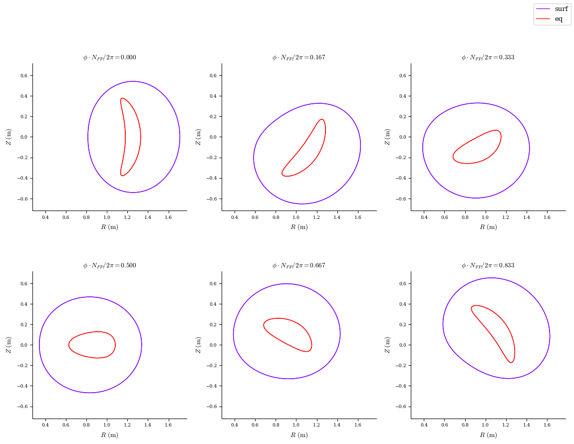
# First, make a constant-offset surface upon which our surface current will lie.
surf = eq.surface.constant_offset_surface(
offset=0.3, # desired offset (m)
M=2, # Poloidal resolution of desired offset surface
N=eq.N, # Toroidal resolution of desired offset surface
grid=LinearGrid(M=8, N=2 * eq.N, NFP=eq.NFP),
)
[18]:
plot_comparison([surf, eq], labels=["surf", "eq"], theta=0, rho=np.array(1.0));
[19]:
# create the FourierCurrentPotentialField object from the constant offset surface we found in the previous cell
surface_current_field = FourierCurrentPotentialField.from_surface(
surf,
I=0,
# manually setting G to value needed to provide the equilibrium's toroidal flux,
# though this is not necessary as it gets set automatically inside the solve_regularized_surface_current function
G=np.asarray(
[
-eq.compute("G", grid=LinearGrid(rho=np.array(1.0)))["G"][0]
/ mu_0
* 2
* np.pi
]
),
# set symmetry of the current potential, "sin" is usually expected for stellarator-symmetric surfaces and equilibria
sym_Phi="sin",
)
surface_current_field.change_Phi_resolution(M=12, N=12)
# solve_regularized_surface_current method runs the REGCOIL algorithm
fields, data = solve_regularized_surface_current(
surface_current_field, # the surface current field whose geometry and Phi resolution will be used
eq=eq, # the Equilibrium object to minimize Bn on the surface of
current_helicity=(
1,
0,
), # pair of integers (M_coil. N_coil), determines topology of contours (almost like QS helicity),
# M_coil is the number of times the coil transits poloidally before closing back on itself
# and N_coil is the toroidal analog (if M_coil!=0 and N_coil=0, we have modular coils, if both M_coil
# and N_coil are nonzero, we have helical coils)
eval_grid=LinearGrid(N=20, M=20, NFP=eq.NFP, sym=True),
source_grid=LinearGrid(N=20, M=20, NFP=eq.NFP),
lambda_regularization=1e-19,
# lambda_regularization determines the complexity of the coils, larger values yield simpler coils at the cost of higher Bn error
vacuum=True, # this is a vacuum equilibrium, so no need to calculate the Bn contribution from the plasma currents
chunk_size=20, # chunk_size controls how many points at a time to evaluate in the biot-savart law,
# setting this to a low number can reduce memory, needed so our notebooks run on Github CI
)
# solve_regularized_surface_current returns a list of FourierCurrentPotentialField objects, one for each lambda, even if a single lambda is passed in
surface_current_field = fields[0]
##########################################################
Calculating Phi_SV for lambda_regularization = 1.00000e-19
##########################################################
chi^2 B = 4.03339e-08
min Bnormal = 3.18663e-11 (T)
Max Bnormal = 4.22072e-06 (T)
Avg Bnormal = 3.90789e-07 (T)
min Bnormal = 3.13440e-11 (unitless)
Max Bnormal = 4.15155e-06 (unitless)
Avg Bnormal = 3.84385e-07 (unitless)
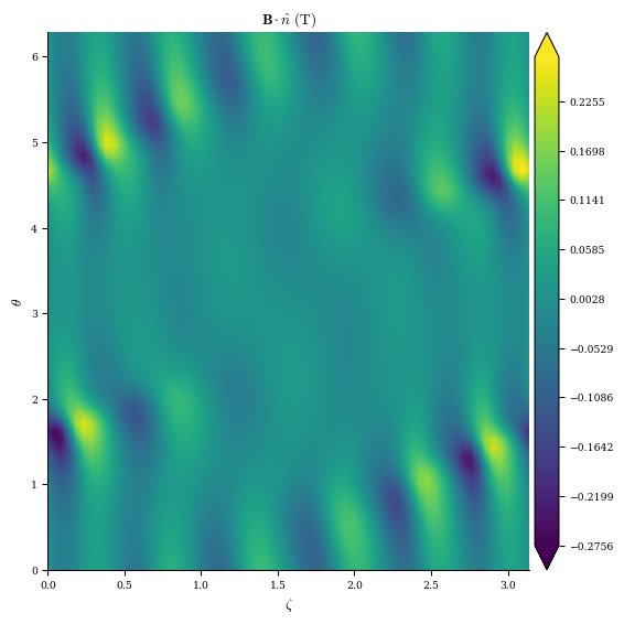
[20]:
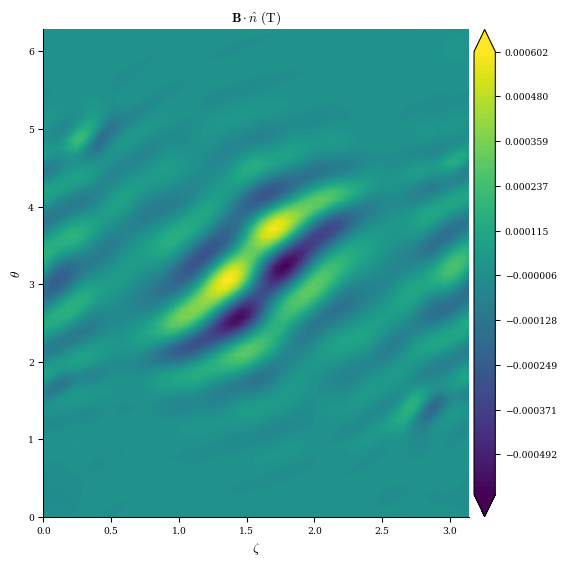
plot_2d(
eq.surface,
"B*n",
field=surface_current_field,
cmap="viridis",
);
[21]:
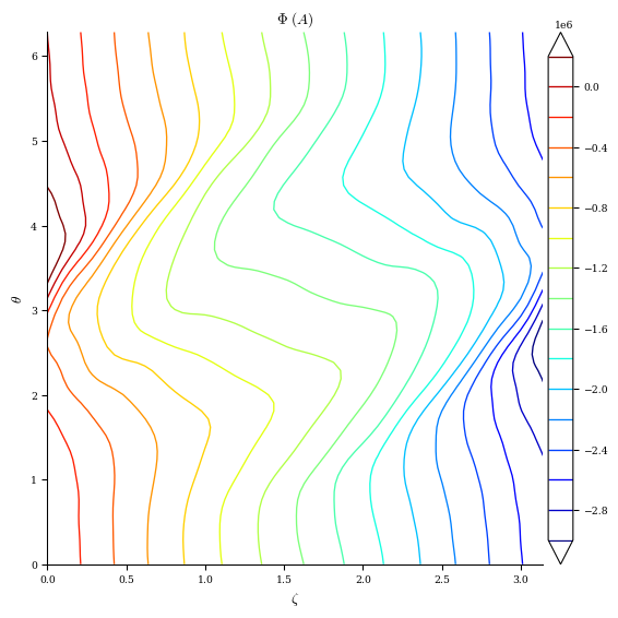
plot_2d(
surface_current_field, "Phi", filled=False, levels=20
); # see how the current potential contours look, these are the coil shapes on the surface
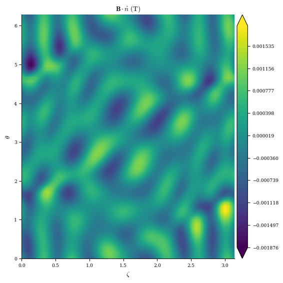
[22]:
# the to_CoilSet method fits the above contours with SplineXYZCoils
coilset_initial_from_regcoil = surface_current_field.to_CoilSet(
num_coils=3, stell_sym=True
)
plot_2d(
eq.surface,
"B*n",
field=coilset_initial_from_regcoil,
cmap="viridis",
)
fig = plot_3d(
eq.surface,
"B*n",
field=coilset_initial_from_regcoil,
field_grid=coil_grid,
grid=plot_grid,
)
fig = plot_coils(coilset_initial_from_regcoil, fig=fig)
fig.show()

[23]:
# we want FourierXYZ to optimize with, so we will fit these with a Fourier series
coilset_initial_from_regcoil = coilset_initial_from_regcoil.to_FourierXYZ(N=10)
plot_2d(
eq.surface,
"B*n",
field=coilset_initial_from_regcoil,
cmap="viridis",
)
fig = plot_3d(
eq.surface,
"B*n",
field=coilset_initial_from_regcoil,
field_grid=coil_grid,
grid=plot_grid,
)
fig = plot_coils(coilset_initial_from_regcoil, fig=fig)
fig.show()
[24]:
# perform optimization now with this coilset as the initial guess, which has better Bn error than our prior guess
weights = {
"quadratic flux": 200,
"coil-coil min dist": 100,
"plasma-coil min dist": 10,
"coil curvature": 500,
"coil length": 2,
}
obj = make_vac_coil_obj(eq, coilset_initial_from_regcoil, weights)
## define our constraints
# we will constrain the current of one coil to avoid the trivial quadratic flux minimizing solution
# of zero coil current
coil_indices_to_fix_current = [False for c in coilset_initial_from_regcoil]
coil_indices_to_fix_current[0] = True
constraints = (
FixCoilCurrent(coilset_initial_from_regcoil, indices=coil_indices_to_fix_current),
)
# Pick an optimizer. For this problem with only linear constraints we can use a regular least squares method.
# if we used the ToroidalFlux constraint we would need to use a constrained optimization method
optimizer = Optimizer("lsq-exact")
(optimized_coilset_initial_from_regcoil,), _ = optimizer.optimize(
coilset_initial_from_regcoil,
objective=obj,
constraints=constraints,
maxiter=100,
verbose=3,
copy=True,
ftol=1e-4,
)
Building objective: Quadratic flux
Precomputing transforms
Timer: Precomputing transforms = 34.0 ms
Building objective: coil-coil minimum distance
Building objective: plasma-coil minimum distance
Building objective: coil curvature
Precomputing transforms
Timer: Precomputing transforms = 5.10 ms
Building objective: coil length
Precomputing transforms
Timer: Precomputing transforms = 4.41 ms
Timer: Objective build = 301 ms
Building objective: fixed coil current
Building objective: fixed shift
Building objective: fixed rotation
Timer: Objective build = 158 ms
Timer: LinearConstraintProjection build = 124 ms
Number of parameters: 191
Number of objectives: 1656
Timer: Initializing the optimization = 597 ms
Starting optimization
Using method: lsq-exact
Solver options:
------------------------------------------------------------
Maximum Function Evaluations : 501
Maximum Allowed Total Δx Norm : inf
Scaled Termination : True
Trust Region Method : qr
Initial Trust Radius : 1.993e+03
Maximum Trust Radius : inf
Minimum Trust Radius : 2.220e-16
Trust Radius Increase Ratio : 2.000e+00
Trust Radius Decrease Ratio : 2.500e-01
Trust Radius Increase Threshold : 7.500e-01
Trust Radius Decrease Threshold : 2.500e-01
------------------------------------------------------------
Iteration Total nfev Cost Cost reduction Step norm Optimality
0 1 7.292e+05 6.737e+02
1 3 2.937e+05 4.354e+05 1.030e-01 2.246e+02
2 4 7.068e+04 2.231e+05 1.757e-01 5.200e+01
3 6 3.595e+04 3.473e+04 8.169e-02 4.537e+01
4 7 9.128e+03 2.682e+04 1.570e-01 1.586e+01
5 10 6.997e+03 2.131e+03 1.770e-02 1.241e+01
6 11 5.576e+03 1.421e+03 3.780e-02 3.076e+01
7 13 4.414e+03 1.162e+03 9.022e-03 7.096e+00
8 14 3.909e+03 5.058e+02 1.893e-02 1.696e+01
9 15 3.087e+03 8.217e+02 1.872e-02 6.920e+00
10 16 2.268e+03 8.190e+02 3.733e-02 1.252e+01
11 17 1.515e+03 7.532e+02 7.344e-02 1.629e+01
12 20 1.216e+03 2.989e+02 3.661e-03 1.457e+01
13 21 1.043e+03 1.731e+02 3.923e-03 2.902e+00
14 22 9.662e+02 7.626e+01 8.641e-03 4.154e+00
15 23 8.985e+02 6.778e+01 1.733e-02 7.431e+00
16 24 7.397e+02 1.587e+02 1.709e-02 5.894e+00
17 25 5.928e+02 1.469e+02 3.426e-02 7.553e+00
18 26 5.654e+02 2.741e+01 3.400e-02 1.585e+01
19 27 3.561e+02 2.093e+02 8.366e-03 2.722e+00
20 28 3.021e+02 5.397e+01 1.683e-02 6.210e-01
21 30 2.798e+02 2.230e+01 8.379e-03 4.654e-01
22 31 2.537e+02 2.609e+01 1.677e-02 3.621e+00
23 32 2.106e+02 4.313e+01 1.666e-02 1.128e+00
24 33 1.588e+02 5.177e+01 3.316e-02 1.276e+00
25 35 1.431e+02 1.569e+01 1.632e-02 1.782e+00
26 36 1.194e+02 2.373e+01 1.626e-02 6.029e-01
27 39 1.179e+02 1.484e+00 1.996e-03 9.057e-01
28 40 1.147e+02 3.216e+00 2.001e-03 6.527e-02
29 41 1.109e+02 3.797e+00 4.006e-03 1.402e-01
30 42 1.043e+02 6.631e+00 7.988e-03 4.133e-01
31 43 1.008e+02 3.494e+00 1.588e-02 1.817e+00
32 44 9.067e+01 1.010e+01 3.856e-03 1.613e+00
33 45 8.253e+01 8.140e+00 7.874e-03 2.938e-01
34 48 8.207e+01 4.566e-01 9.715e-04 7.725e-01
35 49 8.078e+01 1.295e+00 9.678e-04 1.068e-01
36 50 7.943e+01 1.345e+00 1.951e-03 2.458e-02
37 51 7.686e+01 2.568e+00 3.896e-03 4.850e-02
38 52 7.306e+01 3.804e+00 7.762e-03 4.634e-01
39 53 6.494e+01 8.118e+00 1.542e-02 1.132e+00
40 56 6.256e+01 2.384e+00 1.885e-03 2.279e-01
41 57 6.053e+01 2.026e+00 3.781e-03 2.952e-01
42 58 5.699e+01 3.545e+00 7.574e-03 5.389e-01
43 61 5.615e+01 8.373e-01 9.329e-04 4.425e-02
44 62 5.526e+01 8.854e-01 1.879e-03 2.729e-02
45 64 5.483e+01 4.368e-01 9.379e-04 1.593e-02
46 66 5.461e+01 2.165e-01 4.688e-04 1.526e-02
47 67 5.418e+01 4.299e-01 9.377e-04 1.575e-02
48 71 5.417e+01 1.343e-02 2.920e-05 1.492e-02
49 73 5.416e+01 6.686e-03 1.463e-05 1.489e-02
50 74 5.415e+01 1.337e-02 2.927e-05 1.490e-02
51 77 5.415e+01 1.671e-03 3.658e-06 1.490e-02
Optimization terminated successfully.
`ftol` condition satisfied. (ftol=1.00e-04)
Current function value: 5.415e+01
Total delta_x: 1.013e+00
Iterations: 51
Function evaluations: 77
Jacobian evaluations: 52
Timer: Solution time = 30.3 sec
Timer: Avg time per step = 582 ms
==============================================================================================================
Start --> End
Total (sum of squares): 7.292e+05 --> 5.415e+01,
Maximum absolute Boundary normal field error: 9.750e-02 --> 8.500e-04 (T m^2)
Minimum absolute Boundary normal field error: 4.391e-06 --> 1.470e-07 (T m^2)
Average absolute Boundary normal field error: 1.773e-02 --> 1.761e-04 (T m^2)
Maximum absolute Boundary normal field error: 5.777e-01 --> 5.037e-03 (normalized)
Minimum absolute Boundary normal field error: 2.602e-05 --> 8.709e-07 (normalized)
Average absolute Boundary normal field error: 1.050e-01 --> 1.044e-03 (normalized)
Maximum Minimum coil-coil distance: 2.425e-01 --> 1.685e-01 (m)
Minimum Minimum coil-coil distance: 7.577e-02 --> 1.144e-01 (m)
Average Minimum coil-coil distance: 1.439e-01 --> 1.324e-01 (m)
Maximum Minimum coil-coil distance: 4.564e-01 --> 3.170e-01 (normalized)
Minimum Minimum coil-coil distance: 1.426e-01 --> 2.152e-01 (normalized)
Average Minimum coil-coil distance: 2.707e-01 --> 2.491e-01 (normalized)
Maximum Minimum plasma-coil distance: 2.792e-01 --> 4.495e-01 (m)
Minimum Minimum plasma-coil distance: 1.361e-01 --> 3.370e-01 (m)
Average Minimum plasma-coil distance: 2.011e-01 --> 3.793e-01 (m)
Maximum Minimum plasma-coil distance: 1.361e+00 --> 2.191e+00 (normalized)
Minimum Minimum plasma-coil distance: 6.635e-01 --> 1.643e+00 (normalized)
Average Minimum plasma-coil distance: 9.805e-01 --> 1.849e+00 (normalized)
Maximum Coil curvature: 1.095e+01 --> 3.765e+00 (m^-1)
Minimum Coil curvature: -7.688e+00 --> -1.883e+00 (m^-1)
Average Coil curvature: 2.553e+00 --> 1.164e+00 (m^-1)
Maximum Coil curvature: 5.820e+00 --> 2.001e+00 (normalized)
Minimum Coil curvature: -4.086e+00 --> -1.001e+00 (normalized)
Average Coil curvature: 1.357e+00 --> 6.186e-01 (normalized)
Maximum Coil length: 3.393e+00 --> 7.023e+00 (m)
Minimum Coil length: 3.276e+00 --> 5.896e+00 (m)
Average Coil length: 3.339e+00 --> 6.483e+00 (m)
Maximum Coil length: 6.384e+00 --> 1.322e+01 (normalized)
Minimum Coil length: 6.165e+00 --> 1.109e+01 (normalized)
Average Coil length: 6.283e+00 --> 1.220e+01 (normalized)
Fixed coil current error: 0.000e+00 --> 0.000e+00 (A)
==============================================================================================================
[25]:
normalized_field = compute_average_normalized_field(
optimized_coilset_initial_from_regcoil, eq, vacuum=True
)
print(f"<Bn> = {normalized_field:.3e}")
<Bn> = 4.419e-04
[26]:
## visualize the optimized coilset and the normal field error
# passing in eq.surface avoids the unnecessary plasma field computation (as this is a vacuum eq)
plot_2d(
eq.surface,
"B*n",
field=optimized_coilset_initial_from_regcoil,
cmap="viridis",
)
fig = plot_3d(
eq.surface,
"B*n",
field=optimized_coilset_initial_from_regcoil,
field_grid=coil_grid,
grid=plot_grid,
)
fig = plot_coils(optimized_coilset_initial_from_regcoil, fig=fig)
fig.show()
[27]:
plot_field_lines(optimized_coilset_initial_from_regcoil, eq);

Finite Beta
Now let’s get a finite beta stellarator, we’ll use a W7-X example which has \(\beta=2\%\)
[28]:
eq = desc.examples.get("W7-X")
Make Initial Coilset
Again we will initialize with circular coils centered on the equilibrium axis, and with their normal oriented along the axis tangent vector.
[29]:
modular_coilset = initialize_modular_coils(eq, num_coils=3, r_over_a=2.5).to_FourierXYZ(
N=4
)
To this we’ll also add some planar saddle coils. We’ll have coils on both the inboard and outboard side, but only 1 on each side per half-period
[30]:
inner_coils = initialize_saddle_coils(
eq, num_coils=1, r_over_a=1.0, offset=4.0, position="inner"
)
outer_coils = initialize_saddle_coils(
eq, num_coils=1, r_over_a=1.0, offset=4.0, position="outer"
)
Next we’ll combine the modular and windowpane coils into a single MixedCoilSet. This will allow us to optimize both at the same time.
[31]:
coilset = MixedCoilSet(inner_coils, outer_coils, modular_coilset)
# visualize the initial coilset
plot_grid = LinearGrid(
M=40, N=80, NFP=1, endpoint=True
) # a smaller than usual plot grid to reduce memory of the notebook file
fig = plot_3d(eq, "|B|", grid=plot_grid)
fig = plot_coils(coilset, fig=fig)
fig.show()
/CODES/DESC/desc/utils.py:572: UserWarning:
Unequal number of field periods for grid 1 and basis 5.
/CODES/DESC/desc/utils.py:572: UserWarning:
Unequal number of field periods for grid 1 and basis 5.
Optimizing a MixedCoilSet with different types of coils
[32]:
# We'll use the same grid for all the coils. Alternatively, we could use separate grids
# for the windowpane and modular coils.
coil_grid = LinearGrid(N=50)
# we won't define any plasma grid, but instead use the default grid provided by the objective which is usually sufficient
# For coil objectives we can pass lists of bounds, targets, and/or weights to optimize individual coils.
# The lists should broadcast to the tree structure of the coilset.
bounds_length = (
0.0,
[
1.5 * inner_coils[0].compute("length")["length"],
1.5 * outer_coils[0].compute("length")["length"],
1.5 * modular_coilset[0].compute("length")["length"],
],
)
# By setting weights to zero, can exclude certain coils from optimization.
# We optimize CoilCurrentLength (proxy for HTS cost) only for the windowpane coils.
weights_currlength = [1, 1, 0]
obj = ObjectiveFunction(
(
QuadraticFlux(
eq,
field=coilset,
field_grid=coil_grid,
vacuum=False,
weight=200,
bs_chunk_size=10,
),
CoilSetMinDistance(
coilset,
bounds=(0.2, np.inf),
normalize_target=False, # target is already in normalized units
weight=20,
grid=coil_grid,
dist_chunk_size=2, # this helps to reduce peak memory usage, needed to run on github CI
),
CoilLength(
coilset,
bounds=bounds_length,
normalize_target=True, # target in meters
grid=coil_grid,
),
CoilCurvature(
coilset,
# recall that this is signed curvature, in normalized units
bounds=(-1, 2),
normalize_target=False, # target is already in normalized units
weight=30,
grid=coil_grid,
),
CoilCurrentLength(coilset, weight=weights_currlength, grid=coil_grid),
CoilSetLinkingNumber(coilset, weight=500, grid=LinearGrid(N=25)),
LinkingCurrentConsistency(eq, coilset, eq_fixed=True, jac_chunk_size=5),
)
)
# Because the plasma component of the normal field is nonzero, we don't need
# any additional constraints to avoid the trivial solution, but we will include
# constraints to fix the center position of the windowpane coils
constraints = (FixParameters(coilset, params=[{"center": True}, {"center": True}, {}]),)
optimizer = Optimizer("lsq-exact")
(optimized_coilset2,), _ = optimizer.optimize(
coilset,
objective=obj,
constraints=constraints,
maxiter=50,
verbose=3,
copy=True,
)
Building objective: Quadratic flux
Precomputing transforms
Timer: Precomputing transforms = 7.36 sec
Building objective: coil-coil minimum distance
Building objective: coil length
Precomputing transforms
Timer: Precomputing transforms = 230 ms
Building objective: coil curvature
Precomputing transforms
Timer: Precomputing transforms = 9.85 ms
Building objective: coil current length
Precomputing transforms
Timer: Precomputing transforms = 8.16 ms
Building objective: coil-coil linking number
Building objective: linking current
Timer: Objective build = 20.6 sec
Building objective: fixed parameters
Building objective: fixed shift
Building objective: fixed rotation
Timer: Objective build = 174 ms
Timer: LinearConstraintProjection build = 2.85 sec
Number of parameters: 94
Number of objectives: 1702
Timer: Initializing the optimization = 23.8 sec
Starting optimization
Using method: lsq-exact
Solver options:
------------------------------------------------------------
Maximum Function Evaluations : 251
Maximum Allowed Total Δx Norm : inf
Scaled Termination : True
Trust Region Method : qr
Initial Trust Radius : 6.333e+02
Maximum Trust Radius : inf
Minimum Trust Radius : 2.220e-16
Trust Radius Increase Ratio : 2.000e+00
Trust Radius Decrease Ratio : 2.500e-01
Trust Radius Increase Threshold : 7.500e-01
Trust Radius Decrease Threshold : 2.500e-01
------------------------------------------------------------
Iteration Total nfev Cost Cost reduction Step norm Optimality
0 1 2.605e+05 4.171e+02
1 2 6.578e+03 2.539e+05 1.410e+06 4.768e+01
2 5 8.915e+02 5.687e+03 2.512e+05 1.383e+01
3 7 2.322e+02 6.593e+02 1.536e+05 9.082e+00
4 9 1.541e+02 7.814e+01 3.356e+05 1.210e+00
5 10 1.486e+02 5.482e+00 1.100e+05 4.885e+00
6 11 1.448e+02 3.831e+00 3.941e+05 5.852e+00
7 12 1.174e+02 2.735e+01 3.371e+04 1.055e+00
8 13 1.137e+02 3.727e+00 5.106e+04 1.144e+00
9 14 1.096e+02 4.140e+00 5.418e+04 8.943e-01
10 15 1.046e+02 4.938e+00 8.421e+04 1.256e+00
11 16 1.009e+02 3.763e+00 1.623e+05 1.650e+00
12 18 9.532e+01 5.542e+00 3.919e+03 2.445e+00
13 19 9.052e+01 4.794e+00 3.064e+04 1.082e+00
14 20 8.819e+01 2.332e+00 6.333e+04 1.718e+00
15 21 8.592e+01 2.267e+00 5.787e+04 1.927e+00
16 22 8.156e+01 4.362e+00 5.252e+04 7.472e-01
17 24 8.010e+01 1.455e+00 2.117e+04 4.805e-01
18 25 7.881e+01 1.293e+00 4.036e+04 1.090e+00
19 26 7.612e+01 2.694e+00 3.262e+04 1.300e+00
20 28 7.397e+01 2.150e+00 7.152e+03 4.313e-01
21 29 7.308e+01 8.860e-01 1.177e+04 1.379e+00
22 30 7.137e+01 1.708e+00 1.461e+04 1.280e+00
23 31 6.988e+01 1.497e+00 1.791e+04 1.118e+00
24 32 6.929e+01 5.820e-01 1.716e+04 1.216e+00
25 33 6.770e+01 1.594e+00 5.687e+03 9.019e-02
26 34 6.688e+01 8.245e-01 6.533e+03 1.418e-01
27 35 6.568e+01 1.197e+00 1.508e+04 5.092e-01
28 37 6.494e+01 7.354e-01 9.233e+03 5.450e-02
29 38 6.458e+01 3.689e-01 1.237e+04 3.188e-01
Optimization terminated successfully.
`ftol` condition satisfied. (ftol=1.00e-02)
Current function value: 6.458e+01
Total delta_x: 3.555e+05
Iterations: 29
Function evaluations: 38
Jacobian evaluations: 30
Timer: Solution time = 1.21 min
Timer: Avg time per step = 2.43 sec
==============================================================================================================
Start --> End
Total (sum of squares): 2.605e+05 --> 6.458e+01,
Maximum absolute Boundary normal field error: 1.925e+00 --> 1.905e-02 (T m^2)
Minimum absolute Boundary normal field error: 3.726e-15 --> 4.941e-15 (T m^2)
Average absolute Boundary normal field error: 6.300e-01 --> 5.026e-03 (T m^2)
Maximum absolute Boundary normal field error: 2.271e-01 --> 2.248e-03 (normalized)
Minimum absolute Boundary normal field error: 4.396e-16 --> 5.829e-16 (normalized)
Average absolute Boundary normal field error: 7.432e-02 --> 5.929e-04 (normalized)
Maximum Minimum coil-coil distance: 6.720e-01 --> 4.293e-01 (m)
Minimum Minimum coil-coil distance: 6.110e-01 --> 1.924e-01 (m)
Average Minimum coil-coil distance: 6.361e-01 --> 2.518e-01 (m)
Maximum Minimum coil-coil distance: 6.992e-01 --> 4.466e-01 (normalized)
Minimum Minimum coil-coil distance: 6.357e-01 --> 2.002e-01 (normalized)
Average Minimum coil-coil distance: 6.618e-01 --> 2.620e-01 (normalized)
Maximum Coil length: 7.946e+00 --> 1.093e+01 (m)
Minimum Coil length: 3.178e+00 --> 3.018e+00 (m)
Average Coil length: 6.039e+00 --> 7.806e+00 (m)
Maximum Coil length: 8.267e+00 --> 1.137e+01 (normalized)
Minimum Coil length: 3.307e+00 --> 3.140e+00 (normalized)
Average Coil length: 6.283e+00 --> 8.121e+00 (normalized)
Maximum Coil curvature: 1.977e+00 --> 2.203e+00 (m^-1)
Minimum Coil curvature: 7.907e-01 --> -1.618e+00 (m^-1)
Average Coil curvature: 1.265e+00 --> 1.241e+00 (m^-1)
Maximum Coil curvature: 1.900e+00 --> 2.117e+00 (normalized)
Minimum Coil curvature: 7.600e-01 --> -1.555e+00 (normalized)
Average Coil curvature: 1.216e+00 --> 1.193e+00 (normalized)
Maximum absolute Coil current length: 0.000e+00 --> 1.170e+06 (A*m)
Minimum absolute Coil current length: 0.000e+00 --> 7.710e+05 (A*m)
Average absolute Coil current length: 0.000e+00 --> 9.706e+05 (A*m)
Maximum absolute Coil current length: 0.000e+00 --> 7.441e-01 (normalized)
Minimum absolute Coil current length: 0.000e+00 --> 4.903e-01 (normalized)
Average absolute Coil current length: 0.000e+00 --> 6.172e-01 (normalized)
Maximum absolute Coil linking number: 4.754e-11 --> 2.014e-04 (dimensionless)
Minimum absolute Coil linking number: 4.907e-13 --> 4.141e-05 (dimensionless)
Average absolute Coil linking number: 1.035e-11 --> 1.219e-04 (dimensionless)
Linking current error: 1.490e-08 --> 7.884e+07 (A)
Fixed parameters error: 0.000e+00 --> 0.000e+00 (~)
==============================================================================================================
[33]:
normalized_field = compute_average_normalized_field(
optimized_coilset2, eq, chunk_size=10
)
print(f"<Bn> = {normalized_field:.3e}")
<Bn> = 2.614e-02
[34]:
# visualize the optimized coilset and the normal field error
fig = plot_3d(
eq,
"B*n",
field=optimized_coilset2,
field_grid=coil_grid,
grid=plot_grid,
chunk_size=10,
)
fig = plot_coils(optimized_coilset2, fig=fig)
fig.show()
[35]:
# currents in inner saddle coils
optimized_coilset2.coils[0].current
[35]:
[Array(255453.71803704, dtype=float64)]
[36]:
# currents in outer saddle coils
optimized_coilset2.coils[1].current
[36]:
[Array(247259.17866447, dtype=float64)]
[37]:
# current in modular coils
optimized_coilset2.coils[2].current
[37]:
[Array(-86620.11766007, dtype=float64),
Array(-122086.66835804, dtype=float64),
Array(-87551.71972943, dtype=float64)]